
06 Dec 2017
Gradient Descent in Simple NN (ML Series, Part 3)
Note: This post is a WIP. I am leaving it up in its current form for feedback, and will continue to update it, hopefully removing this disclaimer within the week (12/6).
This post builds on Part II of my ML series , and explores what role gradient descent plays in a simple neural network (NN).
I will be working off the simple one layer NN in Andrew Trask’s blog post A Neural Network in 11 Lines of Python (Part I). First, I’m going to review part of Andrew’s posts and explain why this network makes a correct prediction give a certain simple pattern. Next, I’ll create a pattern where the network cannot predict the right answer, and attempt to explain why. In both cases, I will refer back to Part II and build on the purpose of gradient descent. I will be working with this IPython notebook, and it may help to have it open in a separate window.
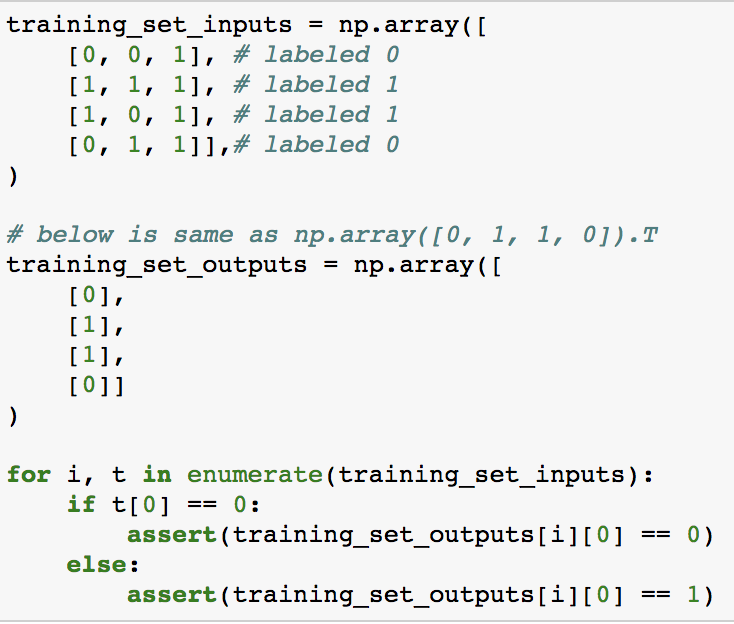
For those unfamiliar with Andrew’s blog post, here’s a quick overview. Andrew creates a fake dataset where each data point is a Python list of three elements. If the first element is 1, then the data point should be labeled 1. If not, it’s labeled 0. A quick visual overview of four example inputs and outputs, which will serve as our training set. Later, we can test the model on the remaining 4 of the eight possible examples of this pattern (2 possibles in each slot -> 2**3):
A Simple and Working NN
Andrew implements a simple neural network in Python using only numpy for some basic utility functions (e.g. taking the dot product of two arrays via np.dot). I want to be clear on what the terminology “implements a simple neural network” means here. The only goal of this exercise is to get three weights - one for each slot - that can be used to make a prediction. Neural network in this case just refers to the methodology for getting these weights. Because the technique to obtain these weights uses parts that are named neurons and activations and layers and is loosely modeled to look like groups of neurons firing, the technique as a whole is a neural network.
Step 1: Randomize Weights
The weights could simply be guessed at. Random guessing does play some role in neural networks (importantly, the guessing is not exactly random and is far beyond the scope of this post), and the initial guess at the final weights leverages np.random.randn. Note that this network uses np.random.seed(1) so outputs are consistent. The first guess at the weights computes 2 * np.random.random((3, 1)) - 1 - the 2 is simply to scale the weights by 2, which are all between 0 and 1. The -1 then forces any weights that were initialized as less than 0.5 to be negative (e.g. 2 * 0.4 - 1 == -0.2).
The first guess at the weights suggests they’re -0.17 (too small), 0.44 (too big) and -0.99 (too small). Because we know that the first slot is the only one that matters, the correct weights are 1, 0 and 0, or some large number and two small numbers. A neural network should move the first weight upward, the second weight downward and the third weight upward.
Step 2: Guess
What is the output when we guess with the weights? The answer to this question is computed via:
predictions = np.dot(training_set_inputs, weights)
The output here is a numpy array of shape (4, 1) (training_set_inputs - four examples of three elements - is (4, 3) and the weights - three “predictors” - are (3, 1)). It represents guesses at the four labels given the four examples in the training set. Of course, these guesses - -2.5, 2.74, 2.95, and -2.73 - are quite far away from the actual labels of 0, 1, 1 and 0.
I want to take a quick second to do some discussion of np.dot. For those with a linear algebra background, feel free to skip this section; I’m an Economics major so np.dot has taken me some time to wrap my head around. The documentation around np.dot makes it sound deceivingly simply:
Dot product of two arrays. For 2-D arrays it is equivalent to matrix multiplication, and for 1-D arrays to inner product of vectors (without complex conjugation). For N dimensions it is a sum product over the last axis of a and the second-to-last of b:
The matrix math explanation makes the most sense here, and the formula you would apply for matrix math does indeed work:
That said, I think the intuition here is important - why are we using np.dot? We know where we want to end up is four predictions, or a numpy array of shape (4, 1). To get each prediction, we need to apply the weights. Getting the sum weighted prediction would look like the below:
- First prediction:
0 * -0.17 + 0 * 0.44 + 1 * -0.99 == -0.99 - Second prediction:
1 * -0.17 + 1 * 0.44 + 1 * -0.99 == -0.73 - Third prediction:
1 * -0.17 + 0 * 0.44 + 1 * -0.99 == -1.17 - Fourth prediction:
0 * -0.17 + 1 * 0.44 + 1 * -0.99 == -0.56
That is all np.dot is doing here. predictions is [[[-0.99977125], [-0.72507825], [-1.16572724], [-0.55912226]]]. The linear algebra intuition for np.dot is a little different, and I have found 3Blue1Brown’s linear algebra series worth watching here (disclaimer: I’m only four videos through). But at least in my minimal machine learning experience, I have found it more useful to stop thinking about rote learning matrix math formulas and referring back to the predictions intuition.
A little terminology here - predictions is really the first hidden layer of the neural network, and also the output layer here as the whole network is only a single input and out layer. In Andrew Ng’s deeplearning course, the step is represented as:
Z1 = W1 * X
where Z1 is the output layer, W1 are weights and X is the training inputs.
Step 3: Apply a Non Linearity and Find Error
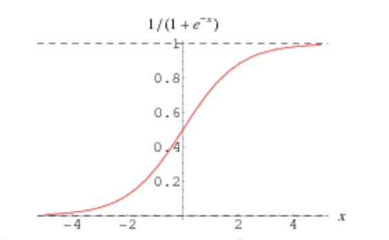
These four numbers from predictions can now be passed through a non-linearity, or function that does not have the same effect on the output as the input is incremented or decremented. Why passing predictions through a non-linearity is important will likely be the subject of another post. For now, I think it’s sufficient to just say that we will pass the four predictions through a function called a sigmoid function that scales them from 0 to 1 and looks like the below:
Again, in Andrew Ng’s deeplearning course, this looks like:
A1 = G(Z1)
where G is the non-linearity (sigmoid function in this example). A1 is called a layer of activations, because the non-linearity is thought to “activate neurons” in the loose brain metaphor.
Step 4: Apply Gradient Descent
Step 5: Update the Weights
Step 6: Repeat
A Simple and Broken NN
This network breaks when changing the rule for inputs and outputs.
